POISSON PROBABILITY DISTRIBUTION (INTRODUCTION)
INTRODUCTION
examples
INTRODUCTION
Probability distributions are used in statistics to understand how likely certain events are. The Poisson probability distribution is used for when we are considering the discrete number of individuals in a given area or events over a period of time. That is, when we make observations what are the probabilities that we see 0, 1, 2, etc. number of individuals or events?
All we need to know is the mean number of individuals in the area we are considering or mean number of events over that period of time. Then, if the assumptions of the binomial distribution are met, the Poisson probability distribution will give us the probability of seeing each particular number of individuals or events.
There are three conditions that must be met in order for a situation to be accurately modeled with a Poisson probability distribution.
The Poisson probability distribution is used for when we are considering the discrete number of individuals in a given area or events over a period of time. That is, when we make observations what are the probabilities that we see 0, 1, 2, etc. number of individuals or events?
All we need to know is the mean number of individuals in the area we are considering or mean number of events over that period of time. Then, if the assumptions of the binomial distribution are met, the Poisson probability distribution will give us the probability of seeing each particular number of individuals or events.
There are three conditions that must be met in order for a situation to be accurately modeled with a Poisson probability distribution.
- 1. The individuals or events occur randomly with respect to one another.
- 2. The individuals or events we are considering should be relatively rare compared to the potential number of observations.
- 3. The probability of an individual occurring in an area, or an event occurring within a time interval, is proportional to the size of the area or the length of time interval.
x is the number of successes we are interested in.
Pr(x) is the probability of seeing x successes.
e is Euler's constant, 2.718281828...
\( \mu \) mean number of individuals or events in a given period of time.
Also, as a reminder, the symbol "!" represents a factorial. A factorial for a number is what we get when we take the number and multiply it by each whole number less than itself (e.g., 2! = 2x1=2, 4!=4x3x2x1=24). By definition 0!=1. If we are using sample data we estimate \( \mu \) with the sample mean \( \bar{x} \) and the equation becomes: $$ Pr(x) = {{\mu^x e^{-\bar{x}}} \over {x!}} $$
TWO EXAMPLES
Before we look at this equation in more detail, let's think of an example of how to use this equation. Imagine we are drawing cards from a deck of cards. We'll draw a card, note what it is, put it back in the deck and draw again. If we do this 52 times we would expect to see each card once on average although obviously for any specific card we may see it more than once or not at all. Let's identify a card like the Ace of Spades and calculate what the odds are that we would draw it no times, once, twice, etc. We can do this long hand by writing out the possible outcomes, but this would quickly become way too big to keep track of. To use the equation above we use an overall mean number of observations of 1. This gives us the following: $$ Pr(0) = {{1^0 e^{-1}} \over {0!}} = {{1} \over {e}} = 0.368 $$ $$ Pr(1) = {{1^1 e^{-1}} \over {1!}} = {{1} \over {e}} = 0.368 $$ $$ Pr(2) = {{1^2 e^{-1}} \over {2!}} = {{1} \over {2e}} = 0.184 $$ $$ Pr(3) = {{1^3 e^{-1}} \over {3!}} = {{1} \over {6e}} = 0.061 $$ $$ Pr(4) = {{1^4 e^{-1}} \over {4!}} = {{1} \over {12e}} = 0.015 $$ $$ Pr(5) = {{1^5 e^{-1}} \over {5!}} = {{1} \over {60e}} = 0.003 $$ $$ Pr(>5) = 0.00059 $$ We can see that the most likely number of observations is the mean which makes sense. We can also see that the probabilities trail off and become small fairly quickly. They never truly reach zero however. We can also look at what this distribution looks like in a figure like the one here - the X-axis is for the number of events that satisfy our requirement (i.e., drawing an Ace of Spades) and the Y-axis shows the probability of seeing each number of successes.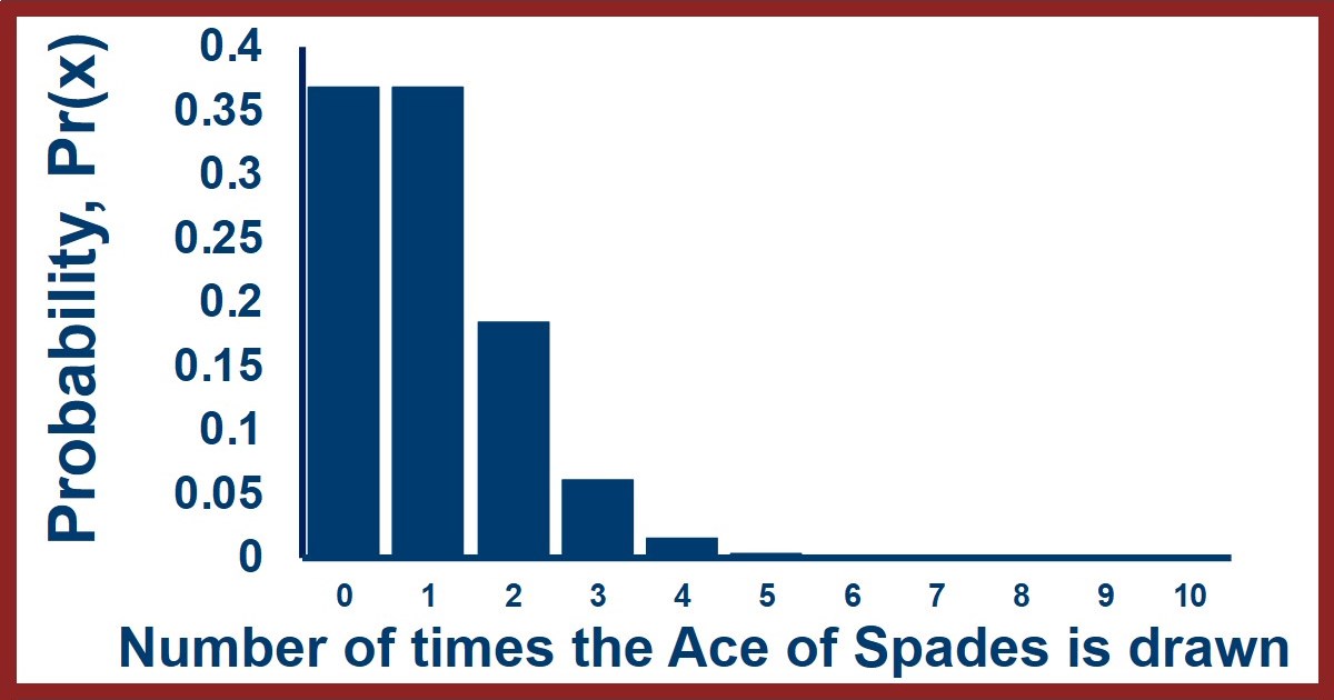
SHORTCUT EQUATION
There is a nice shortcut that allows quick calculation of Poisson probabilities once you know one of them. If you look at the equations for consecutive probabilities: $$ Pr(x) = {{\mu^x e^{-\mu}} \over {x!}} $$ $$ Pr(x+1) = {{\mu^{(x+1)} e^{-\mu}} \over {(x+1)!}} $$ The second can be rearranged to show that it is just first equation, times the mean and divided by x+1, as so: $$ Pr(x+1) = {{\mu^{(x+1)} e^{-\mu}} \over {(x+1)!}} = {{\mu \times \mu^{(x)} e^{-\mu}} \over {(x+1)x!}} = \left({{\mu } \over {x+1}}\right) \left({{\mu^{(x)}e^{-\mu}} \over {x!}}\right) = \left({{\mu } \over {x+1}}\right) Pr(x)$$ For example, in our first example above the first probability was Pr(0)=0.368. Starting from that we would get: $$ Pr(1) = {{1} \over {1}} \times Pr(0) = (1) \times 0.368 = 0.368 $$ $$ Pr(2) = {{1} \over {2}} \times Pr(1) = {{1} \over {2}} \times 0.368 = 0.184 $$ $$ Pr(3) = {{1} \over {3}} \times Pr(2) = {{1} \over {3}} \times 0.184 = 0.061 $$ $$ etc. $$ Which you can see match the values calculated above. Keep in mind that the 1/1, 1/2, and 1/3 fractions on the left in the calculations were the mean divided by the number of observations - if the mean had been 3.2 those values would have been 3.2/1, 3.2/2, and 3.2/3. Using this method can greatly increase the speed of calculating Poisson probabilities. It can also allow you to calculate the full set of probabilities from having any one of the probabilities (i.e., you can use the shortcut to go forwards and backwards).A USEFUL MATHEMATICAL PROPERTY
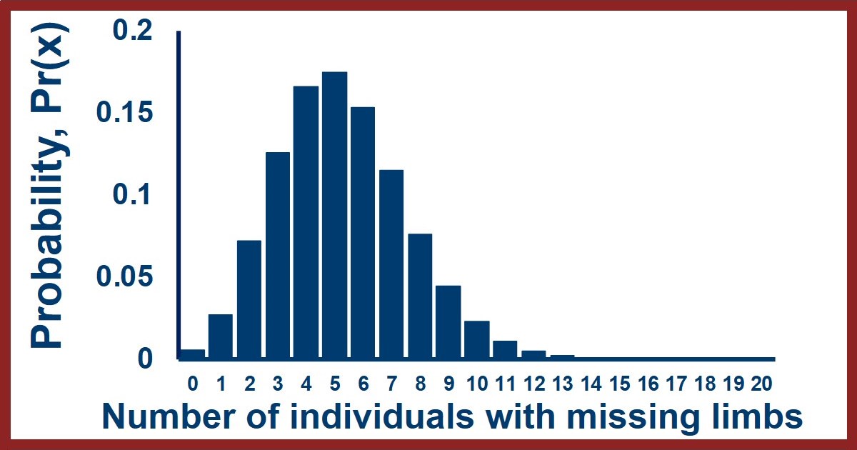
The Poisson distribution has another very convenient mathematical property - its mean is the same as its variance. This property allows us to quickly determine whether a distribution that we think might be a Poisson distribution is one. We can just calculate the mean and variance and compare them. If they are equal we can be confident (but not guaranteed) that the distribution is Poisson, but if the mean and variance are different then we know the distribution is not Poisson. This comparison can be very useful because if we are counting observations that fulfill the assumptions at the top of the page then the distribution should be Poisson - which means that if the distribution doesn't match then one or more of the assumptions isn't true for our data and we've learned something. For example, imagine that we collected data for the number of amputees in a series of towns of size 10,000 across the US. Random factors will cause some of these towns to have fewer or more amputees compared to the mean, but are there non-random factors too? If the risks of being an amputee are random with respect to one another and there are no consistent geographic risks then the distribution should have an equal mean and variance. If we see a difference between the mean and variance however, this would indicate that risk of amputation is not random (perhaps a bad doctor) or that there are geographic differences in risk (more sawmills in certain regions). To facilitate the comparison of the mean and variance in a distribution we think might be Poisson, a value called the "coefficient of dispersion", CD, can be calculated. The CD is the variance divided by the mean: $$ CD = {{variance} \over {mean}} = {{s^2} \over {\bar{x}}} $$ When CD ~ 1.0 the distribution is highly likely to be Poisson and the individuals or events are occurring randomly with respect to one another. There are conceivable cases in which the CD=1 while the distribution isn't Poisson, but these are highly unusual. When CD < 1.0 we say the distribution is "uniform" because the variation is too regular, there is less variation than we expect. Thinking about our first example, this would be like a situation in which we don't shuffle the deck of cards and instead place the card back on the bottom of the deck so we draw it every 52 cards like clockwork. When CD > 1.0 we say the distribution is "clumped" because the variation is too uneven, the observations are more variable than we expect. Thinking about our second example, this would be like a situation in which the military actively recruited from specific towns (resulting in more amputations) while ignoring others (resulting in fewer amputations) so the overall mean is not reflective of the same random process across all the locations.Connect with StatsExamples here
LINK TO SUMMARY SLIDE FROM VIDEO:
StatsExamples-poisson-probability-intro.pdf
TRANSCRIPT OF VIDEO:
Slide 1
Welcome to this introduction to Poisson probability. We'll look at the Poisson probability equation, it's mathematical assumptions, and a few examples of applications. First things first though, This distribution is named after Simeon Denis Poisson so it shouldn't be confused with the English word poison or the French word Poisson which means fish
Slide 2
The Poisson distribution comes from the binomial and it's a special case of the binomial under certain circumstances. If you're familiar with the binomial you'll remember that it describes the probability of seeing X successes in N trials when the success probability is P and is given by the equation P of X equals "N choose X" times the probability of success to the X power times the probability of failure to the N minus X power.
If you don't remember this you can watch our binomial probability videos on this same channel end playlist.
it turns out that when the number of trials gets large and the probability gets small, as a rule of thumb when N is greater than 100 and end times P is less than 10, the binomial probability equation simplifies into the Poisson probability equation .
This equation gives the probability of seeing X successes as the mean number of successes raised to the power X, times E raised the power "negative mean" divided by X factorial.
The two equations shown are for when you have either the population mean or are using a sample mean to calculate your probability
Slide 3
If we look at the Poisson probability equation you'll see that it doesn't have the number of trials or probability of each trial directly in it.
Unlike the binomial which required a set number of trials and a known probability for each trials, the Poisson does not.
Poisson probabilities are used for the probability of seeing X events, or successes, in an area or over a set period of time when we know the mean number of observations or successes .
The potential number of observations can be huge, and even unknowable, so the binomial is not appropriate, but the mean number of observations is often easier to determine.
Slide 4
As mentioned, one typical scenario is calculating the probability of seeing a certain number of events in a given area
For example, if we know the average number of snails per square meter is 3 and we looked in a particular square meter, what are the odds of seeing none at all ?
Another typical scenario would be when we are interested in the probability of seeing events Over a set time.
For example, if we know the average number of deaths in a retirement home is 5 per month, what are the odds of seeing 10 in the same month?
Slide 5
The Poisson probability has three important assumptions.
First, the events occur randomly with respect to one another. This assumption comes directly from the binomial distribution independence assumption.
Second, the events are relatively rare. This is what allows us to replace the binomial equation with the Poisson equation.
Third, the probability of occurrence doesn't change overtime. This assumption comes directly from the binomial distribution's assumption of constant probability
In fact, one way to think about the Poisson distribution is as the limit of the binomial distribution as the probability of each event goes to 0 and the number of trials goes to Infinity.
Slide 6
The Poisson distribution has an incredibly useful property whereby the mean of the distribution is mathematically equal to its variance.
The entire distribution can therefore be specified with one value.
This is useful because this relationship can be used to test hypothesis about whether a distribution we observe is due to Poisson, that is random, process is or not.
If it is then the mean should be equal to the variance
This is usually tested using the coefficient of dispersion represented by the equation to the right where the coefficient of dispersion is equal to the variance divided by the mean and we're usually interested in whether it is equal to 1 or not.
Slide 7
Let's look in more detail at the coefficient of dispersion and what it can tell us. it's equal to the variance divided by the mean and a Poisson distribution would have a coefficient of dispersion of one. The top figure shows a Poisson distribution with the coefficient of dispersion equal to 1
If the variance is less than the mean then the coefficient dispersion is less than one and we term the distribution under-dispersed or uniform.
If we think about what that means in terms of numbers of observations, we see more samples with a number of observations closer to the mean than we expect and fewer samples with numbers of observations far from the mean.
The numbers of successes in our samples are more consistent and similar to each other, which would look like the middle figure. There we see most of the samples having 3 or 4 or 5 observations and very few having two or less or 7 or more.
If the variance is more than the mean then the coefficient dispersion is larger than one and we term the distribution over-dispersed or clumped.
If we think about what that means in terms of numbers of observations, we see fewer samples with a number of observations closer to the mean than we expect and more samples with numbers of observations far from the mean.
The numbers of successes in our samples are not as consistent as we would expect if they were random, which would look like the middle figure. There we see that the samples have a wider range of successes than predicted from a random process.
Slide 8
Another way of visualizing this is to think about what this would look like for our observations in space or time.
The middle figure shows a random distribution of individuals in the square and a random distribution of events along a timeline. We would get a coefficient of dispersion of one if we analyzed the numbers of individuals in randomly chosen areas and the number of events in randomly chosen time periods.
The left figure shows a very nonrandom distribution of individuals or events where they are essentially equally spaced. The numbers of individuals in each region or events per time are much more consistent than we would expect from random processes and we term this under-dispersed or uniform.
The right figure shows a very nonrandom distribution of individuals or events where they are separated into clusters. The numbers of individuals in each region or events per time are much less consistent than we would expect from random processes and we term this over-dispersed or clumped.
Slide 9
Another useful property of the plus on distribution is that consecutive Poisson probabilities are related to each other.
If you look at our equation for the probability, we can separate out a mean in the numerator and the value of X in the denominator and bring that out to the front This would leave the mean raised to one fewer power in the numerator and the factorial of X minus one in the denominator.
But the second part of that equation would be the Poisson probability 4X minus one observations.
therefore the Poisson probability for X is equal to the mean divided by X times the Poisson probability for X minus one.
Slide 10
For example, let's think about if the mean was equal to 3
Slide 11
if the mean is equal to three then the probability of seeing one occurrence is 3 raised to the first power times E to the negative 3 Divided by 1 factorial which would be 0.1494.
Slide 12
The probability of seeing two occurrences is 3 raised to the second power times E to the negative 3 / 2 factorial which would be 0.2240
Slide 13
But if we used our relationship previously, the Poisson probability for 2 should be equal to the mean divided by two, multiplied by the Poisson for 1. This is equal to 3 divided by 2 times the Poisson probability for 1, which is equal to 3 divided by 2 times 0.1494, which is, in fact, equal to 0.2240.
Slide 14
OK, so what applications do we have for the Poisson probability?
One application is that if we know that a process of is random, and we have a mean, then we can predict the probabilities and proportions of numbers or observations
We could then go and measure the numbers of individuals in certain areas to determine whether they are located randomly or due to non-random factors. This sort of thing is done all the time in field ecology for example, where scientists lay out transects and count the number of individuals in each region.
Slide 15
And it's not just for geographic locations that we can look at Poisson probabilities we can look at events overtime as well. If we know that a process is random and we have a mean we can predict probabilities of numbers of events over time.
For example, at the time this video is being made COVID-19 is a brand-new virus still in the early stages of a global pandemic. At this time not much is known about this virus, in particular, how it may be changing over time and why.
The figure shown is a phylogeny, a diagram indicating the ancestry and relatedness of different strains, of covid in different countries. The small circles indicate times when the genetic sequence of that strain changed.
A very important question is whether those genetic changes are just occurring randomly or whether they are occurring non-randomly in response to natural selection. Is there evidence that these genetic changes are because of nonrandom processes like improving its transmissibility or changing its lethality. Or are these changes just random genetic drift?
We can estimate the mean number of changes we see per amount of time, and use that to create predictions for how many changes we expect to see, and compare them to observations for the number of changes we do see.
The Poisson probability provides us with a tool that we can use to better understand the evolution of a deadly disease.
Slide 16
For a final application we can think about one of the scenarios I mentioned at the very beginning of the video.
For example, we expect to see a certain number of deaths each month in a nursing home. The rate of deaths overtime should be constant and the deaths should be independent of one another which would allow us to use the Poisson probability to predict how often we should see different numbers of people dying each month. when there is a month with what seems like an unusually high number of deaths, we can use the poissant to figure out whether it's something we would expect due to random chance or whether there is evidence that there is a non-random factor, like a murderer, in the nursing home.
Comparing unusually large values or apparent patterns to our expectations from randomness has wide applications. For example, the Seti project, a project looking for extraterrestrial life, uses the same sorts of procedures. When they see unusual patterns in their signals they don't instantly get excited, they compare them to how often they would expect to see unusual patterns coming from space.
Zoom out
Having a mathematical and unbiased way of analyzing unusual events is important if we want to make sure we don't get misled. The human brain is hardwired to over interpret noise as pattern and respond emotionally to rare events. Having an approach like the Poisson allows us to mathematically determine whether what we see is genuinely unusual, or what we should expect to see from time to time.
End screen
Feel free to randomly press a button to show your appreciation.
Connect with StatsExamples here
This information is intended for the greater good; please use statistics responsibly.