BINOMIAL PROBABILITY (EXAMPLES)
introduction
EXAMPLES
THE EQUATION
As described on the Introduction to the Binomial Distribution page, when the assumptions of the binomial equation are met, and we know the overall probability of success for each trial (p), we can use the following equation to calculate the probabilities of r successes when we perform k trials: $$ Pr(r) = {k \choose r} p^r (1-p)^{k-r} = {k! \over {r!(k-r)!}} p^r (1-p)^{k-r} $$EXAMPLE 1
Imagine flipping a coin three times and asking what are the probabilities of seeing it come up "heads" zero, once, twice, or three times. To use the binomial equation we use an overall probability of success of p=0.5 and three trials so k=3. This gives us the following: $$ Pr(0) = {3 \choose 0} (0.5)^0 (1-0.5)^{3-0} = {3! \over {0!3!}} (0.5)^0 (0.5)^3 = (1)(1)(0.125) = 0.125 $$ $$ Pr(1) = {3 \choose 1} (0.5)^1 (1-0.5)^{3-1} = {3! \over {1!2!}} (0.5)^1 (0.5)^2 = (3)(0.5)(0.25) = 0.375 $$ $$ Pr(2) = {3 \choose 2} (0.5)^2 (1-0.5)^{3-2} = {3! \over {2!1!}} (0.5)^2 (0.5)^1 = (3)(0.25)(0.5) = 0.375 $$ $$ Pr(3) = {3 \choose 3} (0.5)^3 (1-0.5)^{3-3} = {3! \over {3!0!}} (0.5)^3 (0.5)^0 = (1)(0.125)(1) = 0.125 $$ The probability distribution looks like this with the X-axis for the number of successes and the Y-axis showing the probability of each number of successes when the 3 trials are performed.
EXAMPLE 2
Now let's think about a situation in which we perform 5 trials, each of which has a 25% chance of success. What are the probabilities of seeing 0, 1, 2, 3, 4, or 5 successes? To use the binomial equation we use an overall probability of success of p=0.25 and five trials so k=5. This gives us the following: $$ Pr(0) = {5 \choose 0} (0.25)^0 (1-0.25)^{5-0} = {5! \over {0!5!}} (0.25)^0 (0.75)^5 = (1)(1)(0.237305) = 0.237305 $$ $$ Pr(1) = {5 \choose 1} (0.25)^1 (1-0.25)^{5-1} = {5! \over {1!4!}} (0.25)^1 (0.75)^4 = (5)(0.25)(0.316406) = 0.395508 $$ $$ Pr(2) = {5 \choose 2} (0.25)^2 (1-0.25)^{5-2} = {5! \over {2!3!}} (0.25)^2 (0.75)^3 = (10)(0.0625)(0.421875) = 0.263672 $$ $$ Pr(3) = {5 \choose 3} (0.25)^3 (1-0.25)^{5-3} = {5! \over {3!2!}} (0.25)^3 (0.75)^2 = (10)(0.015625)(0.5625) = 0.087891 $$ $$ Pr(4) = {5 \choose 4} (0.25)^4 (1-0.25)^{5-4} = {5! \over {4!1!}} (0.25)^4 (0.75)^1 = (5)(0.003906)(0.75) = 0.014648 $$ $$ Pr(5) = {5 \choose 5} (0.25)^5 (1-0.25)^{5-5} = {5! \over {5!0!}} (0.25)^5 (0.75)^0 = (1)(0.000977)(1) = 0.000977 $$ The probability distribution looks like this when the 5 trials are performed, note the asymmetric shape because the success probability wasn't 0.5.
EXAMPLE 3
Now let's think about a much bigger scenario in which we perform 12 trials, each of which has a 40% chance of success. What are the probabilities of seeing 0, 1, 2, 3, etc. successes? To use the binomial equation we use an overall probability of success of p=0.4 and k=12. This gives us the following: $$ Pr(0) = {12 \choose 0} (0.4)^0 (1-0.4)^{12-0} = {12! \over {0!12!}} (0.4)^0 (0.6)^12 = {1 \over 1} (1)(0.002177) = 0.002177 $$ $$ Pr(1) = {12 \choose 1} (0.4)^1 (1-0.4)^{12-1} = {12! \over {1!11!}} (0.4)^1 (0.6)^11 = {12 \over 1} (0.4)(0.003628) = 0.017414 $$ $$ Pr(2) = {12 \choose 2} (0.4)^2 (1-0.4)^{12-2} = {12! \over {2!10!}} (0.4)^2 (0.6)^10 = {12x11 \over 2} (0.16)(0.006047) = 0.063852 $$ $$ Pr(3) = {12 \choose 3} (0.4)^3 (1-0.4)^{12-3} = {12! \over {3!9!}} (0.4)^3 (0.6)^9 = {12x11x10 \over 6} (0.064)(0.010078) = 0.141894 $$ $$ Pr(4) = {12 \choose 4} (0.4)^4 (1-0.4)^{12-4} = {12! \over {4!8!}} (0.4)^4 (0.6)^8 = {12x11x10x9 \over 24} (0.0256)(0.016796) = 0.212841 $$ $$ Pr(5) = {12 \choose 5} (0.4)^5 (1-0.4)^{12-5} = {12! \over {5!7!}} (0.4)^5 (0.6)^7 = {12x11x10x9x8 \over 120} (0.01024)(0.027994) = 0.22703 $$ $$ Pr(6) = {12 \choose 6} (0.4)^6 (1-0.4)^{12-6} = {12! \over {6!6!}} (0.4)^6 (0.6)^6 = {12x11x10x9x8x7 \over 720} (0.004096)(0.046656) = 0.176579 $$ $$ Pr(7) = {12 \choose 7} (0.4)^7 (1-0.4)^{12-7} = {12! \over {7!5!}} (0.4)^7 (0.6)^5 = {12x11x10x9x8 \over 120} (0.001638)(0.07776) = 0.100902 $$ $$ Pr(8) = {12 \choose 8} (0.4)^8 (1-0.4)^{12-8} = {12! \over {8!4!}} (0.4)^8 (0.6)^4 = {12x11x10x9 \over 24} (0.000655)(0.1296) = 0.042043 $$ $$ Pr(9) = {12 \choose 9} (0.4)^9 (1-0.4)^{12-9} = {12! \over {9!3!}} (0.4)^9 (0.6)^3 = {12x11x10 \over 6} (0.000262)(0.216) = 0.012457 $$ $$ Pr(10) = {12 \choose 10} (0.4)^10 (1-0.4)^{12-10} = {12! \over {10!2!}} (0.4)^10 (0.6)^2 = {12x11 \over 2} (0.000105)(0.36) = 0.002491 $$ $$ Pr(11) = {12 \choose 11} (0.4)^11 (1-0.4)^{12-11} = {12! \over {11!1!}} (0.4)^11 (0.6)^1 = {12 \over 1} (0.0000419)(0.6) = 0.000302 $$ $$ Pr(12) = {12 \choose 12} (0.4)^12 (1-0.4)^{12-12} = {12! \over {12!0!}} (0.4)^12 (0.6)^0 = {1 \over 1} (0.0000168)(1) = 0.0000168 $$ The probability distribution looks like this when the 12 trials are performed. Note the almost symmetric shape; even though the success probability isn't 0.5, the large number of trials tends to make the binomial distribution resemble the symmetric normal distribution.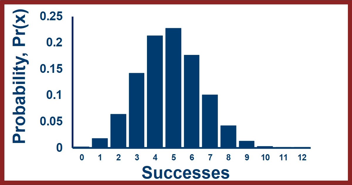
Connect with StatsExamples here
LINK TO SUMMARY SLIDE FROM VIDEO:
StatsExamples-binomial-probability-examples.pdf
TRANSCRIPT OF VIDEO:
Slide 1.
The binomial probability distribution can be very useful, but takes a little practice , so let's do some examples.
Slide 2
First, a quick recap of the basic scenario.
If this is new to you, there is another video on the same channel and playlist that introduces the binomial probability equation.
We have a sample space, or set of possible results from observations, and we classify some events in that sample space as successes and the rest of as failures. This is just an arbitrary label, it doesn't indicate what we want or don't want.
We are thinking about results when we do a bunch of trials, each of which is an observation of an event. We are interested in whether each trial is a success, which is the outcome that fits our criterion, or not for a whole bunch of trials.
The binomial equation calculates the probability of seeing X successes when we do N trials and is shown here.
The probability of observing X successes is "N choose X" times the probability of success raised to the X power times the probability of failure, given by one minus P, raised to the N minus X power
Slide 3
Let's look at our first example and consider a population of frogs in a Lake. We will assume the sex ratio is 0.5 and we will define the success for a trial in which we assess the sex of a chosen frog as that frog being a male.
The success probability for any individual trial is therefore 0.5 and the probability of failure is 1 - 0.5 which is 0.5.
The question that we will address with the binomial probability equation is this. What are the probabilities of collecting six frogs, determining their sexes, and getting a result in which there are zero males, one male, two males etc. from those 6 frogs?
We can look at our binomial probability equation and X will be those numbers 0, 1, two etc and N will be 6. The probability of success will be 0.5.
Plugging those numbers in for the situation where we calculate the probability of seeing 0 males would give us 6 factorial divided by 0 factorial times 6 - 0 factorial, all multiplied by 0.5 to the 0 power times 1 minus 0.5 raised to the 6 minus 0 power.
Slide 4
This first equation is the one we just created and we can see that it simplifies a bit.
The 6 - 0 factorial becomes 6 factorial.
The 0.5 to the zero power becomes one.
The 1 minus 0.5 to the 6 minus 0 power becomes 0.5 to the sixth power
The six factorials cancel to give us one times 1 times 0.5 to the 6th power which equals 0.015625.
We can also look at the probability of observing one male frog in our set of 6. now the probability is equal to 6 factorial divided by 1 factorial times 6 1 factorial all multiplied by zero point 5 to the first power times 1 minus 0.5 raised to the 6 minus 1 power.
The 6 - 1 factorial in the denominator becomes 5 factorial.
The 0.5 to the first power becomes 0.5.
The 1 - 0.5 becomes 0.5 raised to the 6 minus 1 equals 5th power.
The six factorial over 5 factorial reduces down to just six. more on simplifying factorials in fractions in just a second.
In any case, this six is multiplied by zero point 5 times 0.03125 to give us 0.09375.
Slide 5
Before we continue with the binomial probability calculations let's take a look at calculating fractions with factorials.
Let's look at three different ways to represent 6 factorial.
If we write out the whole thing, 6 times 5 times 4 times 3 times 2 times 1 we can see that this is equal to 6 * 5 factorial.
likewise it's equal to 6 times 5 times 4 factorial.
Similarly it's equal to 6 times 5 times 4 times 3 factorial.
This is why the 6 factorial over 5 factorial simplified so easily in the example we just did. 6 factorial is equal to 6 times 5 factorial , the five factorials cancel which just left us with the six.
If we look at the fraction of factorials for N choose X we can see that it will always simplify considerably. if we expand out the factorial in the numerator at some point the entire last part of it will be equal to the second term in the denominator and those can be canceled. This leaves us with fewer terms in the numerator and only one factorial in the denominator.
Let's take a look at how a fraction for a large number of trials could simplify.
For example, "20 choose 7"
Slide 6
"20 choose 7" would be 20 factorial, divided by 7 factorial, times 20 minus 7 factorial. this would be 20 factorial, divided by 7 factorial, times 13 factorial.
If we expand out the numerator, we can see that we would get 20 times 19 times 18 times 17 times 16 times 15 times 14 times 13 factorial.
The 13 factorial in the numerator and denominator would cancel to give us 20 times 19 times 18 times 17 times 16 times 15 times 14 divided by 7 factorial.
We can expand out the factorial in the denominator into 7 times 6 times 5 times 4 times 3 times 2 times 1.
Once we've done this we can see that a few more terms are going to cancel with one another
The 5 and the 3 in the denominator will cancel with the 15 in the numerator.
The 7 and the 2 in the denominator will cancel with the 14 in the numerator.
The 18 in the numerator and the 6 in the denominator can reduce to a three in the numerator.
And the 16 in the numerator and the 4 in the denominator can reduce to a 4 in the numerator
Everything in the denominator has been cancelled and what's left in the numerator is 20 times 19 times 3 times 17 times 4 which equals 77,250.
Slide 7
Returning to our example now , we've already calculated the probability of seeing zero males or one male now let's calculate the probability of seeing two males when we choose six frogs.
That would be "6 choose 2" times 0.5 to the second power times 1 minus 0.5 to the 6 minus 2 power.
For our factorial fraction the six factorial in the numerator and the four factorial in the denominator reduced down to just 6 times 5 in the numerator which would be divided by 2 factorial which is 2 times 1. does
The 0.5 to the second power is 0.25 and the zero point 5 to the 4th power is 0.0625.
When we multiply all this together we get 0.234375
Slide 8
Looking at the binomial probability distribution for this scenario we can see that it is symmetric with the highest probability at three males, that is, three successes.
The sum of all these probabilities will be equal to 1 because there are no other possible results if we do six trials.
And if we wanted to know more complicated results such as the probability of 0 or 1 we could add those probabilities.
Slide 9
Let's look at another example. Consider the game of roulette. In this game there is a wheel that spins and a metal ball that bounces around until it lands in one of the pockets in the wheel. in Europe, where we let is very popular, there are 35 pockets. 18 of them have even numbers , eight of which are red and 10 are black, 18 have odd numbers , ten of which are red and eight are black, and a zero which is colored green.
The simplest kind of bet is to bet on one of the two colors or bet on auto even and if you win you double your money.
Let's think about a scenario in which we spin the wheel three times and we are interested in the probabilities of the ball landing in an even pocket 0, 1, 2, or three times. If we were betting on evens, this kind of calculation may help us figure out what our chances of winning money is.
We can modify our starting binomial probability equation by putting in the 3 for N to get the second equation.
When doing 3 trials, the probability of seeing X successes will be 3 factorial divided by X factorial times 3 minus X factorial all multiplied by the probability of success raised to the X power times 1 minus the probability of success raised to the three minus X power.
Slide 10
To work with our binomial probability equation the first thing we need to do is figure out the probability of success, what is P? Since we are thinking about the probability of getting evens our probability of success will be the 18 even numbered pockets divided by all the pockets which is the 18 evens plus the 18 odds plus the one green 0 which isn't counted as odd or even. doing this division gives us 18 divided by 37 which is 0.486486
Going to our binomial probability equation for three trials and plugging this in our probability of X successes will give the following:
P of X equals 3 factorial divided by X factorial times 3 minus X factorial all multiplied by 0.486486 raised to the X power times 0.513514 raised to the three minus X power.
Slide 11
So, what is our probability of getting 0 , 1, 2, or 3 evens?
Let's do the zero first?
We take our previous equation and plug in zero for X.
The probability of seeing zero evens is 3 factorial divided by 0 factorial times 3 - 0 factorial times 0.486486 to the 0 * 0.513514 to the 3 - 0 power.
This leads to 3 factorial over 1 times 3 factorial so those three factorials will cancel and the whole fraction equals 1.
The 0.486486 to the zero power becomes a 1.
the 0.513514 to the third power is all that's left and that is equal to 0.1354.
Slide 12
Now for the probability of seeing one even.
The probability is 3 factorial divided by 1 factorial times 3 minus 1 factorial all multiplied by 0.486486 to the first power times 0.513514 to the 3 minus 1 power.
The factorial part of the equation is 3 factorial over 1 times 2 factorial and the two factorial cancels out everything except for the three in the numerator.
the 0.486486 the first power is equal to 0.486486 and for the exponent of the second probability term, 3 minus 1 is equal to 2 so the 0.513514 is squared.
Multiplying all of this out gives us 0.3849.
Slide 13
Now for the probability of seeing 2 evens.
The probability is 3 factorial divided by 2 factorial times 3 minus 2 factorial all multiplied by 0.486486 squared times 0.513514 to the 3 minus 2 power.
The factorial part of the equation is 3 factorial over 2 factorial times 1 and the two factorial cancels out everything except for the three in the numerator.
The 0.486486 squared is equal to 0.236669 and for the exponent of the second probability term, 3 minus 2 is equal to 1 so the 0.513514 stays the same.
Multiplying all of this out gives us 0.3646.
Slide 14
Now for the probability of seeing all 3 spins landing as evens.
The probability is 3 factorial divided by 3 factorial times 3 minus 3 factorial all multiplied by 0.486486 cubed times 0.513514 to the 3 minus 3 power.
The factorial part of the equation is 3 factorial over 3 factorial times 0 factorial, which is 1, so everything cancels and the fraction is equal to 1.
The 0.486486 cubed is equal to 0.115136 and for the exponent of the second probability term, 3 minus 3 is equal to 0 so the last term becomes a 1.
Multiplying all of this out gives us 0.1151.
Slide 15
Looking at the binomial probability distribution for this scenario we can see that it is not quite symmetric Because the probability of success is not 0.5. the most likely result is seeing even once but seeing even twice is almost as likely.
The sum of all these probabilities will be equal to 1 because there are no other possible results if we do 3 trials.
We can do a quick mental calculation to see an example of how the casino makes its money. Remember that for bets on even the house doubles the initial wager if you win. If we place the bet on even and then kept it there for all three spins our final amount would be 2 times 2 times 2 equals 8 times what we started with.
That's quite a big gain.
But the probably of that happening is 0.1151 which is less than 1 in 8 which is 0.125. It's possible for us to multiply our initial bet by 8 times but there is a slightly less than one in eight chance of that happening.
That's slightly less is where the casino makes its money.
Slide 16
An interesting aspect of roulette is that it is played differently in Europe and in the United States. in the US there are 2 green pockets, 0 and 00, So there are 36 pockets instead of 35. the payout being double is the same, but the probability of success is now 0.473684 instead of 0.486486.
This creates a slightly different binomial probability distribution for roulette in the United States compared to roulette in Europe. and if you look carefully you can see that the probabilities of winning Are considerably less in the United States.
This may be part of the reason why roulette is much more popular in Europe than it is in the United States
Zoom out
I hope you found these two examples useful in terms of trying to understand how to calculate binomial probabilities, and use the binomial probability distribution to answer questions about the scenario we're studying.
Lots of phenomena we are interested in can be described in a binomial way and the binomial probability equation allows us to predict how often we should see certain kinds of observations.
End screen
Click to show your appreciation if this video was a success.
Connect with StatsExamples here
This information is intended for the greater good; please use statistics responsibly.