BINOMIAL PROBABILITY (INTRODUCTION)

Link to summary slide and video transcript below

INTRODUCTION

Probability distributions are used in statistics to understand how likely certain events are.

The binomial probability distribution is used for when we are considering events we can define as "success" or "failure" - like flipping a coin, assessing whether a study subject did something correctly, or determining whether a trapped animal is male or female. What we define as success or failure is arbitrary as long as we can define all possible outcomes as one or the other.

If we perform a certain number of trials (k) and are interested in the number of successes (r), the binomial probability distribution is the distribution of the expected number of successes out of those trials, Pr(r).

There are four conditions that must be met in order for a situation to be accurately modeled with a binomial probability distribution.

1. There are only two possible outcomes to each trial. This can be done by clearly defining success and calling everything else a failure.
2. There are k trials in the scenario.
3. The probability of a success in each trial is constant throughout the entire set of trials. In other words, any conditions that modify the probability of success can't change as we perform the trials.
4. All trials are independent of one another. In other words, whatever happens in certain trials has no effect on the outcomes of other trials.

If these things are all true, and we know the overall probability of success for each trial (p), we can use the following equation to calculate the probabilities:

$$ Pr(r) = {k \choose r} p^r (1-p)^{k-r} = {k! \over {r!(k-r)!}} p^r (1-p)^{k-r} $$

Where:
r is the number of successes we are interested in.
Pr(r) is the probability of seeing r successes.
k is the number of trials.
p is the probability of success in a single trial.
1-p is the probability of failure in a single trial.
Also, as a reminder, the symbol "!" represents a factorial. A factorial for a number is what we get when we take the number and multiply it by each whole number less than itself (e.g., 2! = 2x1=2, 4!=4x3x2x1=24). By definition 0!=1.

EXAMPLES

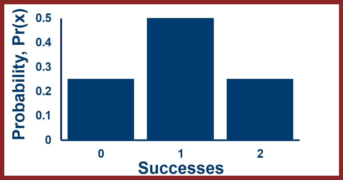
Before we look at this equation in more detail, let's think of an example of how to use this equation. Imagine flipping a coin twice and asking what are the probabilities of seeing it come up "heads" zero, once, or twice.

We can do this long hand by writing out the possible outcomes:
tails then tails
tails then heads
heads then tails
heads then heads
From this we see that the probability of seeing zero successes is 1/4 = 0.25, one success is 2/4 = 0.5, and two successes is 1/4 = 0.25.

To use the equation we use an overall probability of success of p=0.5 and two trials so k=2. This gives us the following: $$ Pr(0) = {2 \choose 0} (0.5)^0 (1-0.5)^{2-0} = 0.25 $$ $$ Pr(1) = {2 \choose 1} (0.5)^1 (1-0.5)^{2-1} = 0.5 $$ $$ Pr(2) = {2 \choose 2} (0.5)^2 (1-0.5)^{2-2} = 0.25 $$ We can see that these values, 0.25, 0.5, and 0.25, match the ones we got from figuring out the probabilities long hand.

We can also look at what this distribution looks like in a figure like the one here - the X-axis is for the number of successes and the Y-axis shows the probability of seeing each number of successes when k trials are performed.

Obviously for this example it is easier to write out the possibiities by hand, but when the probabilities aren't 50/50 or there are lots of trials it quickly becomes much more difficult to do it by writing it out than by using the binomial equation.

Keep in mind that the binomial distribution can be used for situations with success probabilities different from 50% and with many trials - it's not just for flipping coins. This second figure shows a binomial probability distribution for 12 trials with a 40% probability of success. You can see how it's slightly asymmetric, unlike the first figure. Figuring these out longhand would be a nightmare, but it's fairly straightforward with the binomial equation.

See the binomial examples page for more step-by-step examples of calculating binomial probabilities, including this one.

MORE DETAILS

Here's why the equation works. Since the probability of success isn't changing and all the trials are independent, then no one way to get r successes is any more or less likely than any of the others. The binomial works by figuring out the probability of one particular way that k trials can result in r successes (e.g., r successes followed by k-r failures). This is the second part of the equation. And it calculates how many different arrangements there can be for r successes in a string of k trials (e.g., HT and TH are the two options for one success in two trials). This is the first part of the equation with the factorials. Then it combines them - the probability of any particular sequence of successes multiplied by the number of different ways those successes can be ordered.

When we look at the summary statistics for a binomial distribution, the mean, variance and standard deviation will be:

$$ mean = k \times p $$ $$ variance = k \times p \times (1-p) $$

The binomial probability distribution is the most simple probability distribution and it is the basis for the Poisson and normal distributions.

Connect with StatsExamples here

LINK TO SUMMARY SLIDE FROM VIDEO:

StatsExamples-binomial-probability-examples.pdf

TRANSCRIPT OF VIDEO:

Slide 1.

Welcome to this introduction to binomial probability. We'll look at where the binomial probability equation comes from, the mathematical assumptions, and what this can be used for - which is more than just the probabilities of flipping coins although that will be our first example.

Slide 2

OK, let's think about the basic scenario for binomial probability. let's do a set of N trials where we are looking at the outcome of our events in a sample space. Each trial will be an observation of an event. Let's focus on the number of successes, and a success will be an outcome that fits our criterion.
An example of this scenario would be what's shown in the diagram where we are flipping coins and each trial is a coin flip which we are observing. We can define heads as a success and tails as a failure. Success and failure don't mean good or bad, they are arbitrary labels.
The binomial probability method is used when we want to calculate the probability of seeing X number of successes when we do N number of trials.
For example, if we flip a coin N equals 6 times, what's the probability of seeing heads X equals 3 times.

Slide 3

Let's look at our coin flipping example where were flipping a coin 6 times and thinking about the probability of seeing heads three times. We could think of the sample space being half heads and half tails and we are randomly looking at six outcomes in that space.
The probability of getting heads three times would be the number of times we could get would get heads three times out of all the possible results of flipping a coin six times. We could write out all the 2^6 equals 64 possibilities and then look at those to see how many show three heads. Then the probability of getting three heads would be that number divided by 64.

Slide 4

If we do this, we can see that twenty of these possibilities out of the 64 have three heads and three tails.
This is obviously super time consuming and would get impossible very quickly so we need a better way to figure this out.

Slide 5

The better way is the binomial probability procedure. When we're thinking about binomial probabilities there will be 4 assumptions to our scenario.
First, each trial has only two possible outcomes. in the coin flipping example the two outcomes were heads or tails, the coin never landed on its edge or disappeared.
Second, there are N trials. When we do binomial probability calculations we need to know how many trials are being performed .
Third, the probability of success of each trial is constant as we do the trials. This will allow us to use one probability value for all the different trials
Fourth all the trials are independent. This means the results of early trials have no influence on the results of later trials. This also allows us to use the same probability value for all the different trials.

Slide 6

The third assumption, the probability of success being constant, technically means that we would always be doing sampling with replacement in any scenario measuring individuals in a population. If we did sampling without replacement the probability of success would change so our math wouldn't work.

Slide 7

The fourth assumption, the trials being independent, will allow us to use the special ad dition rule. the overall probability of X successes would be the probability of one combination of successes and failures that gives X successes or a second combination of successes and failures that gives X successes or a third combination etc.
Like in the coin flipping example we looked at there were twenty different combinations and we had to consider them all.
If all the trials are independent then we can calculate the probability of combination one or combination two or combination three etc. by calculating the probability of combination one plus the probability of combination two plus the probability of combination three etc.

Slide 8

So we will be calculating the overall probability of X number of successes as the sum of the probabilities of all the different combinations of successes and failures that give X successes.
if the probability of success is constant all the combinations are equally likely.
We could therefore calculate our choice of one combination and then multiply that probability by the number of combinations.
The easiest combination to calculate the probability for would be X successes followed by N minus X failures.
This would be the probability of success raised to the X power times the probability of failure raised to the N minus X power
Since the probability of failure is 1 minus the probability of success, because of our assumption of only two possible outcomes, we can get that final equation where the probability of seeing X successes followed by N minus X failures is the probability of success raised to the X power times the probability of 1 minus success raised to the N minus X power.

Slide 9

That just leaves the question how many combinations are there for two outcomes when we know how many of each outcome there are.

Slide 10

This brings us to something called the binomial coefficient.
If you have N trials and X are successes, then the number of different combinations will be given by the equation to the right.
We read this equation as "N choose X" and it is equal to N factorial divided by X factorial times N minus X factorial.
In case you don't remember, the exclamation point represents a factorial so N! Is "N factorial"
Factorials are calculated by taking the number and multiplying it by each integer less than it down to the number one.
For example 6 factorial is 6 * 5 * 4 * 3 * 2 * 1 which is equal to 720.
Note also that 0 factorial is defined as being equal to 1

Slide 11

So thinking about 3 successes in six trials, this would be "6 choose 3" which is 6 factorial over 3 factorial times 6 minus 3 factorial.
Writing out with this represents gives us 6 times 5 times 4 times 3 times 2 times 1 in the numerator and 3 times 2 times 1 multiplied by 3 times 2 times 1 in the denominator.

Slide 12

A nice feature of fractions with factorials is that often lots of cancellation occurs.
For example, the 3 times 2 times 1 cancels on the top and the bottom and the 3 times 2 times 1 in the denominator is equal to six which cancels with the six in the numerator.
The whole thing reduces nicely down to 5 times 4 equals 20

Slide 13

2 quick things before we continue with the binomial probability calculations.
First, "N choose X" is also written using other nomenclature. All those terms there are also used in different places to represent the same fraction of factorials. When you're reading about binomial probabilities, you'll have to take a little bit of time to figure out which shorthand they're using.
Second, you've actually seen these binomial coefficients calculated before when you did algebra and learned about expanding sums in parentheses that were raised to a different power. You probably learned about Pascal's triangle which allows you to figure out the coefficients, but if you look closely those numbers match the binomial coefficient.
In row six of Pascal's triangle you can see where the 20 comes from for three successes and three failures, it's the coefficient that matches A to the third times B to the third. That's not a coincidence.

Slide 14

Back to our binomial probability calculation we can see it's going to have two parts .
First, will calculate our choice of one combination and that would usually be the combination of X successes followed by N minus X failures
Second, we will multiply that probability by the number of different combinations which comes from N choose X
This gives us the binomial probability equation shown.
The probability of X successes is "N choose X" times the probability of success raised to the X power times 1 minus the probability of success raised to the N minus X power.

Slide 15

So for our original question of flipping a coin 6 times and getting heads three times, the binomial probability equation gives us the probability of getting 3 heads is equal to six choose three times the probability of heads the third power times the probability of tails to the third power.
This is 6 factorial divided by 3 factorial times 6 - 3 factorial times 0.5 to the third power times 0.5 to the 6 - 3 power.
the factorials reduced down to 20 , 0.5 to the third is 0.125, 6 minus 3 is 3 so that's another 0.5 to the third equals 0.125. Multiplying all these together gives us 0.3125.

Slide 16

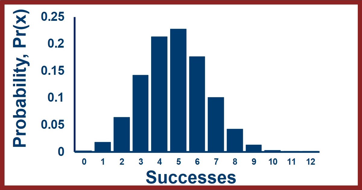
If we repeat these calculations for the other six probabilities, getting 0 heads, getting one heads , etc. we get the probabilities shown here.
One thing to notice is that the sum of all these probabilities add up to one because these are all the possible outcomes from flipping a coin six times.

Slide 17

Let's take a look at what that set of probabilities looks like.
On the X axis we have the number of successes or observations of the outcome we're interested in from zero up to the maximum.
On the Y axis we have the probability of observing each number of successes when we do all of our trials.
A distribution of probability values is called a probability distribution so this is the binomial probability distribution for six trials with a probability of success of 0.5.

Slide 18

One thing to keep in mind is that the binomial probability distribution can have a variety of different probabilities of success.
The probability of success isn't always 0.5 it can be anything from zero to one and the probability distribution would look different for each of them.

Slide 19

Now that we've looked at an example of a single binomial probability distribution let's think about the mathematical properties of the binomial probability distribution in general.
In real world applications of statistics, we are generally taking samples from populations, which means we're interested in what the binomial distribution looks like for those samples.
If we take many samples of size N from a population that exhibits the binomial distribution with success probability P, the expected values for the set of samples will be as shown.
The mean number of successes in those samples will be the number of trials times the probability of success.
The variance of the number of successes in those different samples will be equal to the number of trials times the probability of success times the probability of failure.
For example if we have 100 trials with a probability of success of 0.2 and we look at a bunch of samples the mean number of successes in those samples will be 20 the variance of the number of successes in those samples will be 16 which would give us a standard deviation of 4 and a coefficient of variation of 20%.
If we have 100 trials with the probability of success is 0.5 instead, the mean number of successes in those samples will be 50 the variance of the number of successes in those samples will be 25 which would give us a standard deviation of 5 and a coefficient of variation of 10%.
Notice how the absolute magnitude of the variation in the number of successes increases when the probability is close to 0.5, but the relative variation is less.
If we have the same probabilities, but with more trials, we can see that the absolute magnitude of the variances and standard deviations increase, but the coefficient of variation values indicate that the relative variation decreases.

Slide 20

This is what the binomial probability distributions look like for 100 trials and three different probabilities of success.
Because the product of P and one minus P is maximized for a value of 0.5 we see the largest absolute variation in the samples when the probability of success is 0.5.

Slide 21

This is a figure looking at the relationship between the success probability, the variance of the number of successes seen in samples, and the number of trials in each of those sets of samples. Note that the Y axis labels are not the same in these two figures.
We can see that as the success probability approaches 0.5, the variance in the number of successes is highest and so is the standard deviation. We can also see that as the number of trials increases, the variance increases more quickly than the standard deviation does.

Slide 22

This is especially useful because for binomial and normal distributions approximately 66% of the values are within one standard deviation of the mean and approximately 95% of the values are within 2 standard deviations of the mean.
So if we are taking samples from a population, if we know the population probability of success, we have a quantitative estimate of where we expect most of the numbers of successes in the samples to be.
This relationship can also be used in the other direction. We can test a claim about a population probability by seeing whether the samples, or a sample, looks like we expect if the population probability is what we think it is.

Slide 23

This brings us to applications of the binomial probability distribution.
Remember that there were four assumptions and if they are true the distribution must be binomial.
The first 2 assumptions are usually trivial , but it's the third and fourth that are trickier.
So one application of the binomial probability distribution is that we can measure an observed distribution of samples for which we know the probability of success, or the proportion of an interesting outcome in the population, and compare it to the binomial predicted for that probability.
If these distributions match then the assumptions are probably true and we've learned the probability of success is constant and the trials are independent .
If these distributions don't match then the assumptions are probably not true and we've learned that the probability of success is not constant or the trials are not independent.
Constant probability of success and independence of trials is not always easy to know , but the binomial probability distribution allows us to figure this out.

Slide 24

A second application is the one alluded to earlier, we can test a population proportion hypothesis.
For example, imagine someone makes the claim that a population proportion, that is the success probability, is some value P .
We can test this by taking a bunch of samples of size N from the population.
If the claim is true, the samples should have a mean number of successes equal to N times P with a standard deviation equal to the square root on N times P times 1 minus P
Let's think about a couple of examples up what could happen .
If the claim is that P is equal to 0.34 and we do 100 trials and get a mean number of successes of 33 with a standard deviation of 3, then the 34 we expected is within those 66% and 95% regions we get from 33 plus or minus 3 and 33 plus or minus 6.
However, if the claim is that P is equal to 0.34 and we do 100 trials and get a mean number of successes of 31 with a standard deviation of 1, then the 34 we expected is not within those 66% and 95% regions we get from 31 plus or minus 1 and 31 plus or minus 2.
The binomial probability distribution therefore lets us test claims about probabilities or proportions in populations when we take a set of samples, or even just one sample

Zoom out

Binomial probability can be kind of overwhelming when you first encounter it, but it's not that bad if you go slow and remember what the different parts of the equation represent.
Applications of the binomial probability calculations can be quite useful so it's worth it to learn the method.

End screen

This channel has a companion video that works through a couple of examples of using the binomial distribution linked on the right.

Connect with StatsExamples here

This information is intended for the greater good; please use statistics responsibly.

ABOUT contact privacy credits